Introduction and Executing the Examples

This document describes the use, implementation, and analysis of the GPU accelerated program provided in this tar file. It is not meant as a standalone guide, but is better used as an aid in understanding and using the example code from the tar-file. For resources with in-depth discussions of GPU programming, refer to the listed resources at the end of this document.

The algorithm used for the computationally intensive portion of the example program is a matrix-matrix multiply (C = A*B), referred to by the BLAS naming convention “sgemm” meaning single precision, general matrix multiply. Note that the sgemm implemented in these examples is restricted for simplicity to the square matrix case only, and is a mostly unoptimized simple O(n^3) algorithm.

The tar-file contains the complete source code for all of the examples discussed here, as well as makefiles that will build the executables using either the Gnu or Intel compilers and libraries on Keeneland. Both “accelerated” (meaning that the computation is done by one or more GPUs) and “parallel” (meaning that the work is split between 2+ CPUs or GPUs) examples of the sgemm are provided and discussed. In order to compile using either compiler suite, a symbolic link should be made to the corresponding version of the makefile, followed by running the “make” command.

$ ln -s ./Makefile.keeneland_gnu ./Makefile
$ make

If additional verbose output is desired, the makefiles can be edited to include the preprocessor directive “-DVERBOSE” which will enable additional comments during execution of the various example programs. This is option provides additional debugging messages and is not necessary for general use cases.

After compilation using make, every version of the executable is run in the same way

$ ./exec_name X N

where “exec_name” is the name of the executable, “X” is the number of times the code will generate two random matrices and multiply them together, and “N” is the size of one dimension of the square matrices to be multiplied. Note that all versions of the code assume that all three matrices can be held together in both system and GPU memory. If the executable is run without any arguments, a usage message will be printed that describes the necessary input parameters.

When executed, all versions of the code will give similar output. The first line will describe what the program is doing, based on the command line arguments provided by the user. Next will be timing info that depends on the version of the code and parallelization/acceleration used. Finally, the upper left (6x6) corner of the answer 'C' matrix will be printed. Only the first 6 rows and columns are printed, regardless of the actual size of the matrices computed by the code. Also, only the final 'C' matrix is shown, regardless of how many multiplies were requested using the “X” input parameter to the program.

Serial SGEMM

Program Name: mm

General Notes

This program is the serial, non-accelerated version of the sgemm algorithm that is implemented across all versions of the examples provided.

Both matrices are represented using dynamically allocated single-dimensional arrays, rather than the double square brace syntax, allowed by the C programming language for two-dimensional arrays. This is done to encourage the system to provide contiguous chunks of memory returned by malloc(), which may help improve performance.

Matrix 'B' is generated in column-major order, while matrix 'a' is row-major. This is to allow memory coherency for accessing memory-adjacent elements of both matrices in the innermost multiply loop. Note that this program in fact calculates C = A*B and not C = A*transpose(B).

The timing output that is provided by this and all other examples in the tar-file only takes into account the time spent by the CPU/GPU working on the multiplication of the two matrices. The time spent generating the random input matrices is ignored, as is all other program overhead. This is to provide a more direct comparison between the different methods of accelerating the algorithm of interest (sgemm). In the accelerated and parallel versions, time spent on data movement is accounted for separately. This implies that the wall time for the program execution will differ from the time reported by the program itself.

Compilation Notes

In order to link with the realtime library which provides the timing functions 'clock_gettime()', etc. that are used by the program, '-lrt' must be provided at link time.

$ man clock_gettime

Program Name: mm_mkl

General Notes

This program uses the BLAS sgemm() routine to do the matrix multiply. It is provided both for comparison to the naïve implementation in mm.c, as well as to the GPU accelerated library sgemm() routines provided by CUBLAS and Magma.

BLAS-derived libraries introduce a small difference. Whereas mm.c stored the input and output matrices in row-major form, these libraries assume column-major input and output. For this reason, the random input matrices 'A' and 'B' are generated as transposes compared to mm.c, and the answer 'C' matrix is printed out as a transpose. This allows the same input parameters “X” and “N” to mm.c and mm_mkl.c to output the same matrix elements for consistency checks between programs, as they both ultimately compute the original C = A*B.

If OpenMP is enabled in the MKL library that is being linked to (this is the case on Keeneland), then the number of processors on a node must be specified at runtime. This can be done by using an environment variable, with NP being the number of processors for the MKL routines to use.

$ OMP_NUM_THREADS=NP ./mm_mkl X N

Compilation Notes

Linking against Intel's MKL libraries can be tricky. See the supplied Makefile for hints.

GPU accelerated SGEMM - CUDA and OpenCL

Program Name: mm_cuda

General Notes

Because there is only a single loop in the matrix multiply CUDA kernel, we can get the same type of memory coherency as in mm.c by accessing adjacent elements of each matrix. This is done through the built-in thread addressing capabilities of CUDA exposed through the variables blockIdx.[x,y] and threadIdx.[xy].

There is an explicit synchronization after calling the GPU kernel. This is necessary only for accurate timing purposes; the code will work fine without it. This is because CUDA kernel calls are asynchronous; they return control to the host thread before all compute streams have finished. This will also apply for most libraries that use CUDA (e.g. CUBLAS, Magma).

Compilation Notes

Use the “nvcc” compiler driver to compile source files that end with “.cu” extension. If “.c” is used, nvcc will send the file directly to the C compiler (gcc by default) for compilation, and the CUDA-specific code may not be processed correctly.

Options can be sent to the C compiler by using “-Xcompiler” or “--compiler-options” flag to nvcc. Note that multiple options to be passed must be enclosed in quotes.

Also, it technically shouldn't be necessary to pass the CUDA libs as a linker option to nvcc since it should pick these up automatically, but it doesn't hurt anything.

Program Name: mm_cl

General Notes

This code is split up into two files, the “driver” which should look similar to the other single-node matrix multiply programs, and then the OpenCL bit which is contained in its own file. This is done merely for readability, as the necessary CL code to do all of the initialization can be cumbersome. It also provides an example of how to perform the compilation in such a multiple file situation, as this will typically be desired for more complicated OpenCL and CUDA codes.

There are quite a few steps to get everything set up through OpenCL to use even a simple compute kernel. The OpenCL specification from khronos.org is helpful, and it is ordered in the order of necessary tasks to do when writing an OpenCL program.

Similarly to the CUDA kernel calls, OpenCL calls are asynchronous and require a synchronization only for accurate timing purposes.

There is a complication because OpenCL handles the work block sizes differently than CUDA. There are more sophisticated ways around this issue, but for simplicity here, the matrix is padded so that when it is sent to the GPU, it fits well into the GPU architecture. The other simple way to get around this is to adjust the local worksize so that it evenly divides into the global worksize.

Compilation Notes

Since this program is split into separate files, the driver and CL code are compiled as object files, then linked together. The only other special requirements are to point the compiler where “opencl.h” is found using “-I”, and to link against the corresponding OpenCL libraries. Both of these can be found with the NVIDIA CUDA installation on Keeneland.

GPU Accelerated Libraries - CUBLAS and MAGMA

Program Name: mm_cublas

General Notes

The considerations for matrix structure here are the same as they are for “mm_mkl.” Similarly, the synchronization is necessary for accurate timing as in “mm_cuda.”

Note also that the matrices are copied to the GPU in the same way as a CUDA program. Essentially, the CUBLAS call takes the place of a custom CUDA kernel call.

Compilation Notes

This program is compiled identically to a regular CUDA program.

Program Name: mm_magma

General Notes

This program is almost identical to “mm_cublas,” except for the way the data is transferred to the GPU. Instead of using the native CUDA calls, the magma library provides its own magma_ssetmatrix().

Compilation Notes

The regular C compiler is used rather than nvcc, as there is no explicit GPU code in the mm_magma.c source file. In addition, the code must be linked against the magma libraries, as well as the CUDA libraries for the GPU memory allocation routines.

In order to use an up-to-date version of the Magma library on Keeneland, the source code can be downloaded from the link under the “Resources” section at the end of this document. After unpacking, the “make.inc” file provided in the tar-file related to this document can be copied into the base Magma directory, then simply typing “make” will build Magma. The location of the Magma directory can then be referenced in the linked Makefile that builds the sgemm examples.

GPU Acceleration Using Directives

Program Name: mm_acc

General Notes

There are a few considerations that need to be made to use the PGI implementation of the OpenACC directives. Any memory blocks that will be used within the directives need to have the “restrict” keyword added to their declarations.

In order for the compiler to properly recognize the available parallelization in the algorithm, the program must use 2D arrays and loop over the separately dimensions of the arrays. It seems that using 1D arrays and accessing the memory non-sequentially confuses the auto-parallelization recognition in the compiler.

Compilation Notes

In this example, the PGI compiler is used to provide support for the OpenACC directives. On Keeneland, it is most easily accessed through the “programming environment” modules.

$ module swap PE-intel PE-pgi

In order to enable the ACC interpreter, the compiler should be invoked with the command line option “-ta=nvidia,time” This tells the compiler to use the NVIDIA GPU as a target. The optional “time” target enables some extra runtime output about the performance of the code running on the GPU. Another useful command line option is “-Minfo” which will show compile-time information about the parallelizations being done.

Parallelization - MPI

Program Name: mm_mpi

General Notes

All MPI-enabled programs in this example tar-file must be run with at least 2 MPI threads because they use the master/worker model where one thread as “master” delegates the work evenly between all of the remaining “worker” threads.

The 'A' matrix is split up, with an equal number of rows from 'A' being sent to each worker, as well as all of 'B'. Then, each worker sends back its computed portion of 'C', along with timing information which is then averaged by the master thread and reported.

Compilation Notes

When using mpicc and having the correct modules loaded, the linking against MPI as done in the Makefile is optional. However, it should make for a more robust executable, that is, that it will still run against those specific MPI libraries even if the runtime environment is not set up identically as at compile-time (e.g. different modules are loaded).

Program Name: mm_mpi_mkl

General Notes

This cuts up the work among the worker tasks, then each worker simply uses the BLAS “sgemm()” routine to do a single precision general matrix multiply.

As mentioned previously, BLAS (and related) introduces a difference – these routines expect everything to be stored and used in column-major order. For this reason, the program generates the transpose of A and B, and split the work among the processes by sending columns of B (whereas before, it had sent rows of A). The final answer still comes out to be the original C = A*B.

If OpenMP is enabled in the MKL library that is being linked to (this is the case on Keeneland), then the number of processors on a node must be specified at runtime. This can be done by using an environment variable, with Nomp being the number of processors for each of the Nthr MPI threads to use.

$ OMP_NUM_THREADS=Nomp mpiexec -n Nthr ./mm_mpi_mkl X N

Compilation Notes

Compilation here is similar to the serial mm_mkl.c case. See the supplied makefiles for details.

Parallel GPU Accelerated SGEMM – CUDA and OpenCL across MPI

Program Name: mm_mpi_cuda

General Notes

This version works conceptually the same as “mm_cuda,” except that the 'A' matrix is split up and each worker thread calls its own CUDA kernel to work on its portion of the computation. To do this, the program makes a few CUDA calls to auto-detect the number of available GPUs on the node, then it mods the MPI worker taskid by the number of GPUs to grab them in a round robin manner. This should work correctly because, as per the openmpi faq, openmpi schedules the threads by filling a node with available threads, then moving on to the next (see www.open-mpi.org/faq/?category=running#mpirun-scheduling).

As an example, if the job script specifies

nodes=2:ncpu=4:gpus=4

and the program is run with

mpirun -n 7

then MPI tasks 1-4 will execute on the first node, with tasks 5-7 on the second node.

Compilation Notes

When combining MPI/CUDA, it is easiest to compile the CUDA code with 'nvcc' into an object file, then link with the rest of the C code using mpicc.

Note that it is not strictly necessary to compile driver as an object before linking – this could be done in one step.

However, when linking in this way, it is necessary to explicitly link against the CUDA libs because the linking step is being done by 'mpicc' and not 'nvcc' which had taken care of it automatically in the case of 'mm_cuda'.

Program Name: mm_mpi_cl

General Notes

The strategy here is largely the same as with “mm_mpi_cuda.”

Similarly to the serial case in mm_cl, matrix padding is used to fit the problem on the GPU properly. Unlike with mm_cl, the number of worker tasks is taken into account so that each gets the same number of rows before padding. The upper bound on the padding will be on the order of BLOCK_SIZE*numworkers in the worst case.

Compilation Notes

Compilation is also very similar to “mm_mpi_cuda.”

Parallel GPU Accelerated libraries – CUBLAS and MAGMA across MPI

Program Name: mm_mpi_cublas

General Notes

This is a straightforward extension of “mm_cublas,” with the similar caveats about matrix structure and work division as was present in “mm_mpi_mkl.”

Compilation Notes

Again, we have split up the MPI and CUDA (here CUBLAS) portions of the code to make compilation simpler.

Program Name: mm_mpi_magma

General Notes

Similar to the serial case, this program is almost identical to the mm_mpi_cublas case, except for the function calls to transfer the data to and from the GPU.

Compilation Notes

Compilation is identical to the serial mm_magma.c case, except that mpicc is used here.

As explained in the mm_magma section of this document, in order to use an up-to-date version of the Magma library on Keeneland, the source code can be downloaded from the link under the “Resources” section at the end of this document. After unpacking, the “make.inc” file provided in the tar-file related to this document can be copied into the base Magma directory, then simply typing “make” will build Magma. The location of the Magma directory can then be referenced in the linked Makefile that builds the sgemm examples.

Performance Analysis

One of the main motivations for using GPU acceleration is to increase performance, so understanding some issues that affect performance as well as simple performance analyses can aid in achieving this goal.

Weak Scaling

Not all problems are suited for GPU acceleration. The GPU can process large amounts of homogeneous data very quickly, but there may not be much gain if the problem is not large enough. This issue can be seen in a plot that shows the weak scaling of a program – how the program scales as the input size varies.

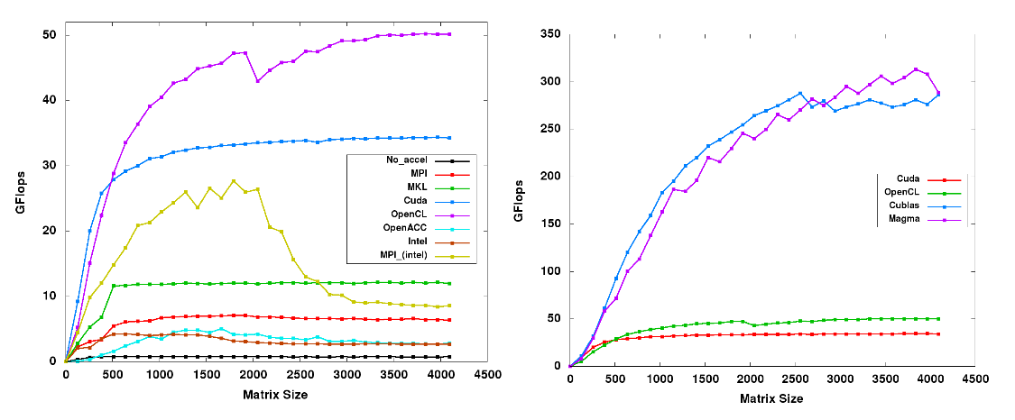
In this plot, not only is the relative performance of each program shown, but also the minimum input size required for top performance.

Strong Scaling

Because the GPU is a parallel computing resources, strong scaling is also an important consideration. Strong scaling graphs show the performance of a program as more computational resources are added. Ideal strong scaling is a linear increase with unity slope. However, this is rarely achieved because the cost of data transfer between the parallel resources can negate a portion of the speedup.

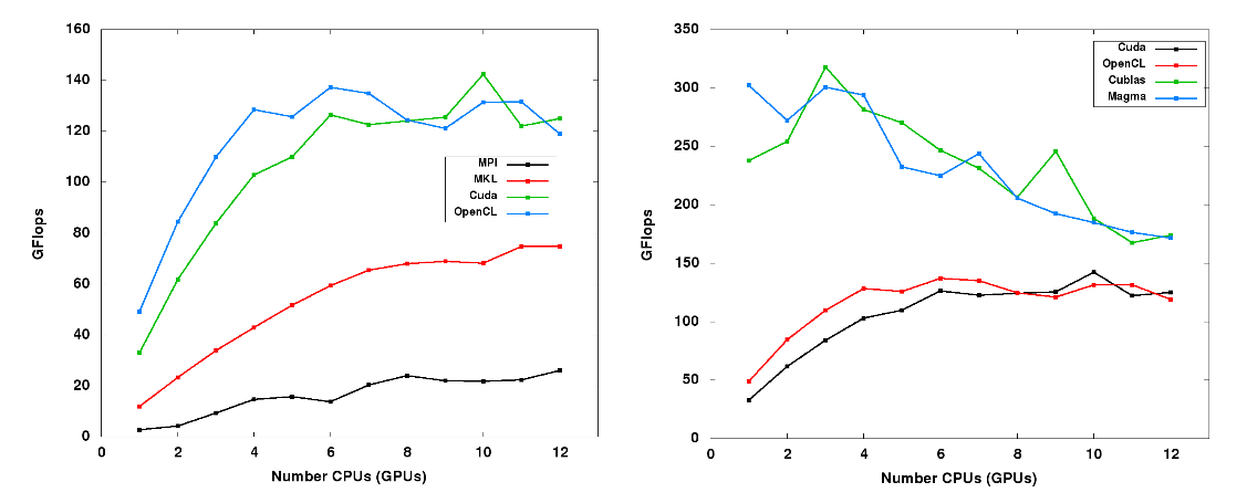
Plots like this one hint at a threshold, after which it is no longer an advantage to keep adding computational resources because the cost of communication is negating the extra help.

Compilers and Compiler Optimizations

Although not the case for the example programs discussed here, if a program has significant non-GPU portions, then the compiler and its optimizations could make a difference in the overall performance of the code.

This graph shows the relative performance of the serial, non-GPU sgemm program when compiled with different compilers/optimizations. There are a couple of points to note: 1) The Intel compilers perform the best on Keeneland for this particular example, presumably because Keeneland uses Intel processors and the Intel compilers are better able to target and exploit the architecture. 2) The level of optimization does not in general make a large difference for many cases. This could be due to the simplicity of the algorithm – being just 3 nested loops that do a multiply and an add. Therefore, this algorithm may not present ample opportunity to the compiler for more sophisticated optimizations after loop unrolling and/or vectorization.

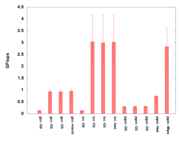
Lastly, there are many issues related to compiler optimization and tuning that are beyond the scope of this document that could be relevant, especially for more complicated algorithms and implementations.

GPU Optimization Strategies

Architecture Considerations

Correctly allocating the GPU resources and optimally arranging the data on the GPU can have an effect on getting the best performance out of a GPU program. This involves, among other things, specifying the correct number of “grids” and “blocks” to use the NVIDIA CUDA terminology.

Memory

Just as is the case with CPUs, GPU devices have a heterogeneous memory layout. However, the developer must take care to exploit this layout to get the potential performance gains. These types of optimizations include using modified algorithms (e.g. tiling algorithms for sgemm) in order to have fewer memory accesses, and using shared memory for faster accesses.

Asynchronous Execution and Communication Hiding

As seen in the strong scaling results above, performance can be improved if the effects of communication can be mitigated. Fortunately, most GPU devices have at least some capability for asynchronous execution, which means that it can be performing two or more tasks simultaneously. For example, a kernel could be doing calculations on the GPU device, while at the same time data is moved back and forth in preparation for the next computationally intensive section of the program to be executed on the GPU.

Resources

CUDA/CUBLAS

- NVIDIA's CUDA developer documentation (http://www.nvidia.com/content/cuda/cuda- documentation.html)

- NVIDIA SDK examples (http://www.nvidia.com/content/cuda/cuda-downloads.html)

OpenCL

- Khronos group online documentation (http://www.khronos.org/opencl/resources)

- OpenCL specification (http://www.khronos.org/registry/cl/)

MAGMA

- Innovative Computing Laboratory (ICL) Magma website (http://icl.cs.utk.edu/magma/index.html)

Books

There are many well-written books available about CUDA programming, and a few about OpenCL. These are easily found through large internet book sellers.

Future Work

These are a few ideas for how this project could be continued in a useful way.

Stepwise Optimization Examples

Each of the programs in this set can be optimized in some way; most of them would gain a lot of performance from hand optimizations. It could be instructive to do these optimizations one at a time, starting with the simplest, and provide separate examples that clearly show each type of optimization.

Additional Examples

Additional examples that take a similar approach to the sgemm already presented could be used for comparison by someone who is starting out in learning to write GPU programs. More complicated linear algebra kernels and algorithms from other computational areas (e.g. n-body, graph theory, grid methods, etc.) could illuminate other strategies and issues that arise with GPU programming, as well as provide a wider base of knowledge from which a student could produce their own custom GPU algorithm.

OpenACC Optimization and Parallelization

There is quite some room for improvement in the OpenACC implementations. At the time of this writing, there is no working parallel OpenACC enabled compiler. A skeleton code is provided, but has not been thoroughly tested.

Also, in both the serial and parallel implementations, there are additional directives that can possibly be employed to improve performance of the OpenACC acceleration. These include specifying the data locality traits, as well as allocating the GPU resources in a reasonable way that matches the algorithm and size of the input data.

Profiling and Debugging

Profiling and debugging tools can make tuning code for optimal performance more efficient. Profiling/debugging tools that can be used with GPU-accellerated codes can be explored and used on the provided programs to show the developer how to get started with some more advanced profiling/debugging tasks.